Monetary Policy Sentiment index
Sentiment Analysis of Monetary Policy Communication
Daniel H. Vedia-Jerez
This page contains the Python code for my Medium blog publication entitled: “Sentiment Analysis of Monetary Policy Communication: Part I”. Visit Medium for its analysis and countinuing with its following part on Covid-19 and Monetary Policy sentiments in the Euro Area.
Here, we add all the Python code for making the Sentiment Analysis, measure the Sentiment index for the Monetary Policy for the four main central banks of the world: Federal Reserve, European Central Bank, Bank of England, and Bank of Japan.
Data sources
The sources of the data are access free and can download it, all the communique were downloaded from the BIS Central bank speeches, and for some cases, we use the specific Central Bank pages, especially for the case of Japan and England, more specifically for the Governors Mr. T. Fukui and Lord King respectively.
The interest rate and the GDP growth rate were also downloaded from each Central bank.
Note. - The code example for this blog post is only for the case of the Bank of England.
Importing the main libraries and modules
import codecs
import datetime as dt
import os
import pickle
import re
import matplotlib.pyplot as plt
For tokenizing sentences
import nltk
import numpy as np
import pandas as pd
from tqdm import tqdm_notebook as tqdm
from tone_count import *
The tone_count module is available here.
The tone_count has to functions, the first just determines if preceding word is a negation word, and the last and main important counts the positive and negative words with negation check (the previous function). Account for simple negation only for positive words. Simple negation is taken to be observations of one of negate words occurring within three words preceding a positive words.
nltk.download("punkt")
plt.style.use("seaborn-whitegrid")
[nltk_data]   Downloading package punkt to
[nltk_data]   C:\Users\canut\AppData\Roaming\nltk_data...
[nltk_data]   Package punkt is already up-to-date!
Open the dataframe and other requisites, in this case two additional files, the list of sentiments of Loughran and McDonald Sentiment Word List. I add negation check as suggested by Loughran and McDonald (2011). That is, any occurrence of negate words (e.g., isn’t, not, never) within three words preceding a positive word will flip that positive word into a negative one.
boe = "DB/boe_pickle"
infile = open(boe, "rb")
boe = pickle.load(infile)
lm = "E:data\\list_sent"
infile = open(lm, "rb")
lmdict = pickle.load(infile)
neg = "E:data\\negate"
infile = open(neg, "rb")
negate = pickle.load(infile)
print(len(boe))
124
Measuring the elapse time, although the database is not extensive, the tone_count module took 23 seconds.
Next, we measure the Wordcount, the number of positive words, and the number of negative words.
import time
start = time.time()
temp = [tone_count_with_negation_check(lmdict, x) for x in boe.text]
temp = pd.DataFrame(temp)
end = time.time()
print(end - start)
23.20803737640381
boe["wordcount"] = temp.iloc[:, 0].values
boe["NPositiveWords"] = temp.iloc[:, 1].values
boe["NNegativeWords"] = temp.iloc[:, 2].values
Sentiment Score normalized by the number of words.
boe["sentiment"] = (
    (boe["NPositiveWords"] - boe["NNegativeWords"]) / boe["wordcount"] * 100
)

boe["Poswords"] = temp.iloc[:, 3].values
boe["Negwords"] = temp.iloc[:, 4].values
boe.head()
| text | Index | wordcount | NPositiveWords | NNegativeWords | sentiment | Poswords | Negwords | |
|---|---|---|---|---|---|---|---|---|
| date | ||||||||
| 2008-01-22 | Speech given by Mervyn King, Governor of the B... | 0 | 2292 | 89 | 122 | -1.439791 | [growth, more, most, largest, increasing, grow... | [default, crisis, losses, collapse, losses, fe... |
| 2008-03-19 | Sovereign Wealth Funds and Global Imbalances S... | 1 | 4047 | 136 | 138 | -0.049419 | [growth, higher, higher, up, benefited, most, ... | [imbalances, default, questions, failings, imb... |
| 2008-03-31 | Extract from a speech by Mervyn King, Governor... | 2 | 1482 | 45 | 38 | 0.472335 | [more, stability, achieve, more, more, enable,... | [default, interference, down, low, lower, fall... |
| 2008-04-20 | Monetary Policy and the Financial System Remar... | 3 | 2820 | 43 | 107 | -2.269504 | [more, rise, rise, above, rise, transparency, ... | [default, turmoil, serious, challenges, tighte... |
| 2008-06-21 | How Big is the Risk of Recession? Speech given... | 4 | 3834 | 150 | 127 | 0.599896 | [good, delighted, most, opportunity, valuable,... | [risk, recession, default, strong, slow, weake... |
pl = pd.DataFrame()

pl["date"] = pd.to_datetime(boe.index.values, format="%Y-%m-%d")
pl["b"] = pl["date"].apply(lambda x: x.strftime("%Y-%m"))
print(pl["b"])
boe = pd.merge(boe, pl, left_on="Index", right_index=True)
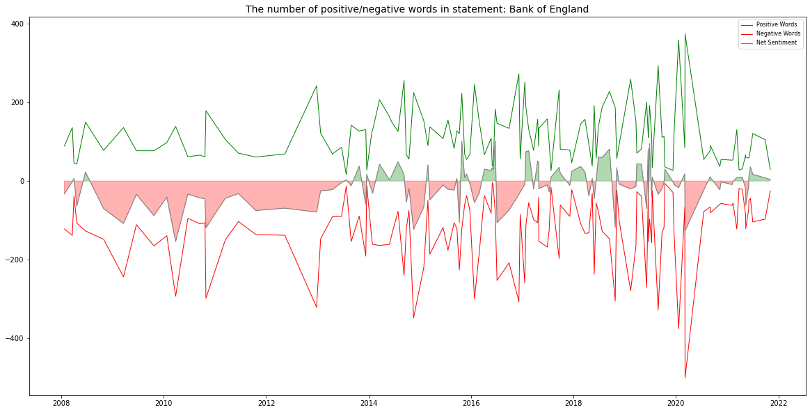
Finally, we plot the number of Positive, Negative words and the Net Sentiment index.
import matplotlib.dates as mdates
NetSentiment = boe["NPositiveWords"] - boe["NNegativeWords"]
fig = plt.figure(figsize=(20, 10))
ax = plt.subplot()

plt.plot(boe.date, boe["NPositiveWords"], c="green", linewidth=1.0)
plt.plot(boe.date, boe["NNegativeWords"] * -1, c="red", linewidth=1.0)
plt.plot(boe.date, NetSentiment, c="grey", linewidth=1.0)

plt.title(
    "The number of positive/negative words in statement: Bank of England", fontsize=14
)
plt.legend(
    ["Positive Words", "Negative Words", "Net Sentiment"], prop={"size": 8}, loc=1
)

ax.fill_between(
    boe.date,
    NetSentiment,
    where=(NetSentiment > 0),
    color="green",
    alpha=0.3,
    interpolate=True,
)
ax.fill_between(
    boe.date,
    NetSentiment,
    where=(NetSentiment <= 0),
    color="red",
    alpha=0.3,
    interpolate=True,
)

years = mdates.YearLocator()  # every year
months = mdates.MonthLocator()  # every month
years_fmt = mdates.DateFormatter("%Y")
ax.xaxis.set_major_locator(years)
ax.xaxis.set_major_formatter(years_fmt)
ax.xaxis.set_minor_locator(months)
# Minor ticks every month.
fmt_month = mdates.MonthLocator()
ax.xaxis.set_minor_locator(fmt_month)
ax.xaxis.set_major_formatter(mdates.DateFormatter("%Y-%m"))
datemin = np.datetime64(boe.date[0], "Y")
datemax = np.datetime64(boe.date[-1], "Y") + np.timedelta64(1, "Y")
# plt.xticks(range(len(pl.b)), pl.b, rotation = 'vertical',fontsize=8)
ax.set_xlim(datemin, datemax)
ax.grid(True)
plt.show()
Net Sentiment analysis
NetSentiment = boe["NPositiveWords"] - boe["NNegativeWords"]
Normalize data
NPositiveWordsNorm = (
    boe["NPositiveWords"] / boe["wordcount"] * np.mean(boe["wordcount"])
)
NNegativeWordsNorm = (
    boe["NNegativeWords"] / boe["wordcount"] * np.mean(boe["wordcount"])
)
NetSentimentNorm = NPositiveWordsNorm - NNegativeWordsNorm
fig, ax = plt.subplots(figsize=(15, 7))
ax.plot(boe.date, NPositiveWordsNorm, c="green", linewidth=1.0)
plt.plot(boe.date, NNegativeWordsNorm, c="red", linewidth=1.0)

plt.title("Counts normalized by the number of words", fontsize=16)
plt.legend(
    ["Count of Positive Words", "Count of Negative Words"], prop={"size": 12}, loc=1
)
years = mdates.YearLocator()  # every year
months = mdates.MonthLocator()  # every month
years_fmt = mdates.DateFormatter("%Y")
# format the coords message box
datemin = np.datetime64(boe.date[0], "Y")
datemax = np.datetime64(boe.date[-1], "Y") + np.timedelta64(1, "Y")
# plt.xticks(range(0,len(pl.b),6), pl.b, rotation = 45,fontsize=8)
ax.set_xlim(datemin, datemax)
# format the coords message box
ax.format_xdata = mdates.DateFormatter("%Y-%m-%d")
ax.grid(True)
plt.show()
import nltk.data
tokenizer = nltk.data.load("tokenizers/punkt/english.pickle")
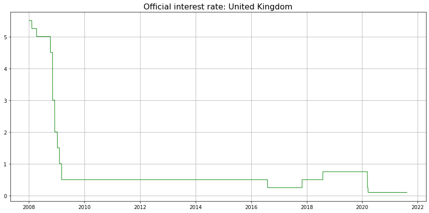
Loading interest rates DB
boerate = pd.read_excel(r"DB/int.xlsx")
boerate["Date"] = pd.to_datetime(boerate.Date.values, format="%Y-%m-%d")
boerate.set_index(["Date"])
boerate.fillna(method="ffill", inplace=True)
boerate.info()
selected_columns = boerate[["Date", "Official Rate"]]
rate_df = selected_columns.copy()
rate_df.rename(columns={"Official Rate": "Rate"}, inplace=True)
datetime_series = pd.to_datetime(rate_df["Date"])
datetime_index = pd.DatetimeIndex(datetime_series.values)
rate_df = rate_df.set_index(datetime_index)
print(rate_df.index)
fig, ax = plt.subplots(figsize=(15, 7))
plt.title("Official interest rate: United Kingdom", fontsize=16)
ax.plot(rate_df.Date, rate_df["Rate"].values, c="green", linewidth=1.0)
ax.grid(True)
plt.show()

Adding interest rate decision
boe["RateDecision"] = None
boe["Rate"] = None
for i in range(len(boe)):
    for j in range(len(rate_df)):
        if boe.date[i] == rate_df.Date[j]:
            boe["Rate"][i] = float(rate_df["Rate"][j + ]
We check for NAS, it is possible due to spare days in the communique database.
boe[boe["Rate"].isna()]
boe["Rate"].fillna(method="ffill", inplace=True)
for i in range(len(boe) - 1):
    if boe["Rate"][i] == boe["Rate"][i + 1]:
        boe["RateDecision"][i] = 0
    elif boe["Rate"][i] < boe["Rate"][i + 1]:
        boe["RateDecision"][i] = 1
    elif boe["Rate"][i] > boe["Rate"][i + 1]:
        boe["RateDecision"][i] = -1
boe.head(5)
| text | Index | wordcount | NPositiveWords | NNegativeWords | sentiment | Poswords | Negwords | date | b | RateDecision | Rate | |
|---|---|---|---|---|---|---|---|---|---|---|---|---|
| date | ||||||||||||
| 2008-01-22 | Speech given by Mervyn King, Governor of the B... | 0 | 2292 | 89 | 122 | -1.439791 | [growth, more, most, largest, increasing, grow... | [default, crisis, losses, collapse, losses, fe... | 2008-01-22 | 2008-01 | -1 | 5.50 |
| 2008-03-19 | Sovereign Wealth Funds and Global Imbalances S... | 1 | 4047 | 136 | 138 | -0.049419 | [growth, higher, higher, up, benefited, most, ... | [imbalances, default, questions, failings, imb... | 2008-03-19 | 2008-03 | 0 | 5.25 |
| 2008-03-31 | Extract from a speech by Mervyn King, Governor... | 2 | 1482 | 45 | 38 | 0.472335 | [more, stability, achieve, more, more, enable,... | [default, interference, down, low, lower, fall... | 2008-03-31 | 2008-03 | 0 | 5.25 |
| 2008-04-20 | Monetary Policy and the Financial System Remar... | 3 | 2820 | 43 | 107 | -2.269504 | [more, rise, rise, above, rise, transparency, ... | [default, turmoil, serious, challenges, tighte... | 2008-04-20 | 2008-04 | 0 | 5.25 |
| 2008-06-21 | How Big is the Risk of Recession? Speech given... | 4 | 3834 | 150 | 127 | 0.599896 | [good, delighted, most, opportunity, valuable,... | [risk, recession, default, strong, slow, weake... | 2008-06-21 | 2008-06 | -1 | 5.25 |
boe[boe["RateDecision"].isna()]
boe["RateDecision"].fillna(method="ffill", inplace=True)
Save as pickle for the next part
rate_des_pickle = "DB/rate_boe"
rate_des_o = open(rate_des_pickle, "wb")
pickle.dump(boe, rate_des_o)
rate_des_o.close()
In case you need save as an excel spreadsheet.
boe.to_excel("E:\\GitRepo\\CB speeches\\data\\sent_BOE.xlsx",
    sheet_name="BOE", engine="xlsxwriter")
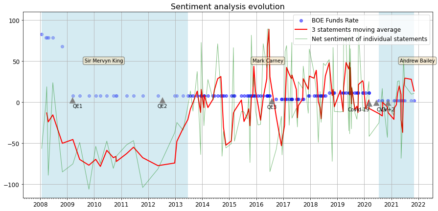
Finally, we prepare the code for the last graph considering each governor’s period in office, also it is included the official interest rate of the Bank of England.
Final plot: Sentiment index and official interest rate
Speaker window
King = np.logical_and(boe.index > "2003-07-01", boe.index < "2013-07-01")
Carney = np.logical_and(boe.index > "2013-07-01", boe.index < "2020-03-15")
Bailey = np.logical_and(boe.index > "2020-03-16", boe.index < "2028-03-16")
Speaker = np.logical_or.reduce((King, Bailey))
Moving Average
Window = round(0.025 * len(boe))
CompToMA = NetSentimentNorm.rolling(Window).mean()
cmin, cmax = None, None
if CompToMA.min() < NetSentimentNorm.min():
    cmin = CompToMA.min()
else:
    cmin = NetSentimentNorm.min()
if CompToMA.max() > NetSentimentNorm.max():
    cmax = CompToMA.max()
else:
    cmax = NetSentimentNorm.max()
Final Plotting Data
import datetime
import matplotlib.dates as mdates
import matplotlib.transforms as mtransforms
fig, ax = plt.subplots(figsize=(15, 7))
plt.title("Sentiment analysis evolution", fontsize=16)

ax.scatter(boe.date, boe["Rate"] * 15, c="blue", alpha=0.5)
ax.plot(boe.date, CompToMA, c="red", linewidth=2.0)
ax.plot(boe.date, NetSentimentNorm, c="green", linewidth=1, alpha=0.5)
ax.legend(
    [   "BOE Funds Rate", str(str(Window) + " statements moving average"),
        "Net sentiment of individual statements"
    ],
    prop={"size": 12},
    loc=1,)

years = mdates.YearLocator()  # every year
months = mdates.MonthLocator()  # every month
years_fmt = mdates.DateFormatter("%Y")

# Set X-axis and Y-axis range

ax.xaxis.set_major_locator(years)
ax.xaxis.set_major_formatter(years_fmt)
ax.xaxis.set_minor_locator(months)

ax.xaxis.set_major_locator(years)
ax.xaxis.set_major_formatter(years_fmt)
ax.xaxis.set_minor_locator(months)

# format the coords message box

ax.format_xdata = mdates.DateFormatter("%Y-%m-%d")
ax.grid(True)
ax.tick_params(axis="both", which="major", labelsize=12)

# Fill Speaker

trans = mtransforms.blended_transform_factory(ax.transData, ax.transAxes)
theta = 0.9
ax.fill_between(boe.index, 0, 10, where=Speaker, facecolor="lightblue", alpha=0.5, transform=trans)

# Add text
props = dict(boxstyle="round", facecolor="wheat", alpha=0.5)
ax.text(
    0.15,
    0.75,
    "Sir Mervyn King",
    transform=ax.transAxes,
    fontsize=10,
    verticalalignment="top",
    bbox=props,)
ax.text(
    0.56,
    0.75,
    "Mark Carney",
    transform=ax.transAxes,
    fontsize=10,
    verticalalignment="top",
    bbox=props,)
ax.text(
    0.92,
    0.75,
    "Andrew Bailey",
    transform=ax.transAxes,
    fontsize=10,
    verticalalignment="top",
    bbox=props,)

# Add annotations

q1 = mdates.date2num(datetime.datetime(2009, 3, 15))
q2 = mdates.date2num(datetime.datetime(2012, 7, 13))
q3 = mdates.date2num(datetime.datetime(2016, 8, 1))
q4 = mdates.date2num(datetime.datetime(2020, 3, 10))
q41 = mdates.date2num(datetime.datetime(2020, 6, 13))
q42 = mdates.date2num(datetime.datetime(2020, 11, 18))

arrow_style = dict(facecolor="black", edgecolor="white", shrink=0.05)
ax.annotate(
    "QE1",
    xy=(q1, 6),
    xytext=(q1, -8),
    size=10,
    ha="left",
    verticalalignment="bottom",
    arrowprops=dict(arrow_style, shrink=0.05, ls="--", color="gray", lw=0.5),)
ax.annotate(
    "QE2",
    xy=(q2, 6),
    xytext=(q2, -8),
    size=10,
    ha="center",
    verticalalignment="bottom",
    arrowprops=dict(arrow_style, shrink=0.05, ls="--", color="gray", lw=0.5),)
ax.annotate(
    "QE3",
    xy=(q3, 5),
    xytext=(q3, -9),
    size=10,
    ha="center",
    verticalalignment="bottom",
    arrowprops=dict(arrow_style, shrink=0.05, ls="--", color="gray", lw=0.5),)
ax.annotate(
    "Covid-19",
    xy=(q4, 2),
    xytext=(q4, -12),
    size=10,
    ha="right",
    verticalalignment="bottom",
    arrowprops=dict(arrow_style, shrink=0.05, ls="--", color="gray", lw=0.5),)
ax.annotate(
    "CV+",
    xy=(q41, 3),
    xytext=(q41, -12),
    size=10,
    ha="left",
    verticalalignment="bottom",
    arrowprops=dict(arrow_style, shrink=0.05, ls="--", color="gray", lw=0.5),)
ax.annotate(
    "CV+2",
    xy=(q42, 3),
    xytext=(q42, -12),
    size=10,
    ha="center",
    verticalalignment="bottom",
    arrowprops=dict(arrow_style, shrink=0.05, ls="--", color="gray", lw=0.5),)

plt.show()

The end…